A Quick Introduction

PyZX can be installed as a package using pip:

pip install pyzx

If you wish to use the demo notebooks or benchmark circuits, then the repository can be cloned from Github.

The best way to get started if you have cloned the repository is to run the Getting Started notebook in Jupyter. This page is meant to give you an overall view of what can be done with pyZX, but the notebook explains all this and more in much more detail.

Warning

The newer JupyterLab as opposed to the older Jupyter Notebook uses a different framework for widgets which is currently not compatible with the widgets used in PyZX. It is therefore recommended that you use the classic notebook interface. If you are using JupyterLab you can find this interface by going to ‘Help -> Launch Classic Notebook’.

Let’s start by importing the library:

>>> import pyzx as zx

For all the examples in this documentation we will assume you have imported PyZX in this manner.

Quantum circuits in PyZX are represented by the Circuit class. Files in the supported formats (QASM, QC, Quipper) can easily be imported into PyZX:

circuit = zx.Circuit.load("path/to/circuit.extension")

The circuit file-formats supported by Circuit.load are curently qasm, qc or quipper.

PyZX tries to automatically figure out in which format the circuit is represented. The generate module supplies several ways to generate random circuits:

>>> circuit = zx.generate.CNOT_HAD_PHASE_circuit(qubits=4,depth=20,clifford=True)

If you are running inside a Jupyter notebook, circuits can be easily visualized:

>>> zx.draw(circuit)

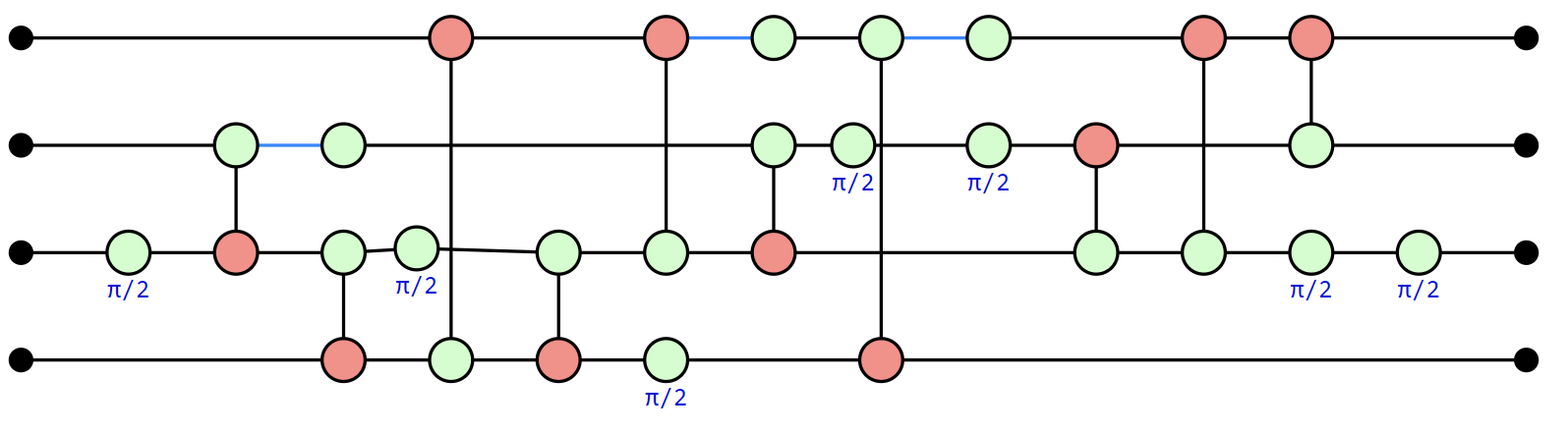
The default drawing method is to use the D3 Javascript library. When not running in a Jupyter notebook zx.draw returns a matplotlib figure instead. The green and red nodes represent the Z- and X- phase gates respectively. In PyZX, Hadamard gates are stored as edges between vertices, which here are shown as blue lines.

There are two main data structures in PyZX, Circuits and Graphs. A Circuit is essentially just a list of gates. The above is an example of a Circuit:

>>>print(circuit.gates)
[CNOT(2,3), CNOT(0,1), CNOT(1,3), CNOT(1,2), CNOT(1,3), S(0), S(1), S(3), HAD(2), HAD(3), CNOT(2,1), HAD(3), CNOT(2,0), S(3), CNOT(1,3), S(3), HAD(0), HAD(1), CNOT(3,1), CNOT(3,2)]

Most of the functionality in PyZX works on Graphs instead, which directly represent ZX-diagrams (the drawing function zx.draw above for instance first converted the circuit into a Graph before drawing it). ZX-diagrams are represented by instances of BaseGraph. To convert a circuit into a ZX-diagram, simply do:

g = circuit.to_graph()

Let us use one of the built-in ZX-diagram simplification routines on this ZX-diagram:

>>> zx.clifford_simp(g)  # simplifies the diagram
>>> g.normalize()  # makes it more presentable
>>> zx.draw(g)

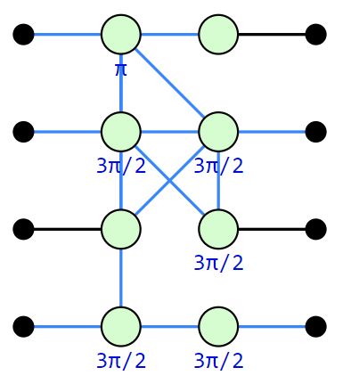
The same circuit, but rewritten into a more compact ZX-diagram. The blue lines represent edges which have a Hadamard gate on them.

Internally, a ZX-diagram is just a graph with some additional data:

>>> print(g)
Graph(16 vertices, 21 edges)

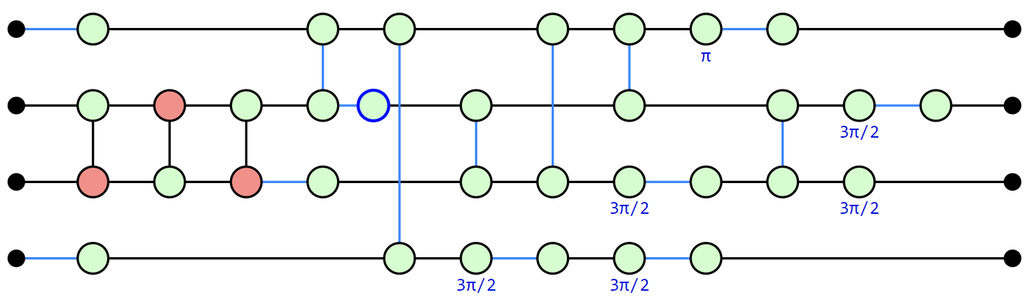
The simplified ZX-diagram above no longer looks like a circuit. PyZX supplies some methods for turning a Graph back into a circuit:

>>> c = zx.extract_circuit(g.copy())
>>> zx.draw(c)

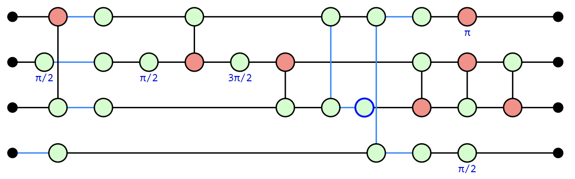
This extraction procedure is sometimes not as good at keeping the number of two-qubit gates low, and will sometimes increase the size of the circuit. PyZX also supplies some Circuit-level optimisers that more consistently reduce the size of the circuit (but are less powerful):

>>> c2 = zx.optimize.basic_optimization(c.to_basic_gates())
>>> zx.draw(c2)

To verify that the optimized circuit is still equal to the original we can convert them to numpy tensors and compare equality directly:

>>> zx.compare_tensors(c2,g,preserve_scalar=False)
        True

We can convert circuits into one of several circuit description languages, such as QASM:

>>> print(c2.to_qasm())
OPENQASM 2.0;
include "qelib1.inc";
qreg q[4];
rz(0.5*pi) q[1];
h q[1];
rz(0.5*pi) q[1];
cx q[2], q[0];
h q[2];
h q[3];
h q[0];
cx q[0], q[1];
sdg q[1];
cx q[2], q[1];
cz q[0], q[2];
h q[2];
cz q[0], q[3];
h q[3];
rz(0.5*pi) q[3];
h q[0];
x q[0];
cx q[1], q[2];
cx q[2], q[1];
cx q[1], q[2];

PyZX can also be run from the command-line for some easy circuit-to-circuit manipulation. In order to optimize a circuit you can run the command:

python -m pyzx opt input_circuit.qasm

For more information regarding the command-line tools, run python -m pyzx --help.

This concludes this tutorial. For more explanation and an example of optimizing a predefined circuit look at the Getting Started notebook. For more information about the simplification procedures see List of simplifications. The different representations of the graphs and circuits is detailed in Importing and exporting quantum circuits and ZX-diagrams. How to create and modify ZX-diagrams is explained in ZX-diagrams in PyZX and how to modify them.